Joining in QGIS
Details: This is using the QGIS long-term release as of 2/22/20 Using qgis long-term release as of 2/22/20
We’re going to start from two shapefiles and one dataset:
- A shapefile obtained from the Phoenix Police Department of polygons containing the grids used by the police to classify crimes.
- A shapefile obtained from the Phoenix Police Department’s open government site showing the locations of police stations as points.
- A data file of all 911 calls to the police from the city’s open government site. I queried it to get the number of calls by grid, understanding that about 10 percent of the calls fall between boundaries and are not counted. This is just for the purpose of illustration.
Plug-ins
Like packages in R, plug-ins take common tasks and automate them for you. Two very common plug-ins are “MMQIS” and “HCQMIS”. Each of these has tasks for geocoding and for base maps that will help.
What you might want to do
- Make a map based on data you have that you can join to the database: Same unit of analysis.
- Aggregate data based on a larger variable – example, points to census tracts, then count them that way - based on location rather than a matching field.
- Apply information from one unit of analysis to another. For example, find out information about a precinct based on block groups, or get information about a police grid based on census tracts. Often using Census for this but not always.
Important preprocessing
Know your projections
Each map should come with information about its projection and datum. “Datum” refers to which system is used as a starting point. I the US, this is sually NAD 1983 or NAD 1927 (North American Datum). The difference is that measuring got better over the years, so they started over in 1983 when they could measure. The difference is usually within a few meters in practice, but assuming the wrong datum can make everything look slightly off.
“Projection” refers to where and how the attributes look on a flat surface. Most local governments save all of their data in a consistent projection. In Phoenix, it’s usually “1983 HARN State Plane Arizona Central FIPS 0202 Feet” . (Some states only have one projection - states with large areas have several. Most places I live use the state plane measured in meters, but I’ve found feet is more common in the West. ). Sometimes they won’t tell you what it is – they’ll just give you a code called “EPSG”. For example, the police points came as Spatial Reference: 2868. If you look that up on a web Spatial Reference list, it comes back to 1983 NAD 83 HARN Arizona Central.
This is important. Sometimes the files are missing or incorrect, and your map can show up in Africa somewhere when you overlay it with another.
Unit of Analysis
If you want to put data together with maps, they have to
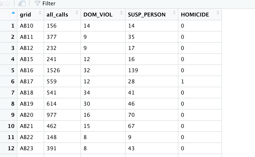
a) Have the same unit of analysis. That is, there can only be one row for each attribute in the shapefile. In our case, we can only have one row per grid. That means that unlike other times we deal with data, we’re going to want to have a short, wide dataset – not a long narrow one. You can preprocess your data using pivot_wider in R, or you can create different csv files for each attribute you want to explore. If your file is big, you’ll want to try to combine them. In our case, I created an R program to create a data file that would match up with the shapes. This involved getting one row for each grid, and combining grids that had more than four characters. In this case, I’m interested in domestic violence, homicides and suspicious person calls:
  calls_by_type_2019 <-
      police_calls %>%
      filter (year(call_date ) == 2019) %>%
      mutate (call_type = case_when ( str_detect( final_radio_code, "^647") ~ "SUSP_PERSON",
                         str_detect (final_radio_code, "^451") ~ "HOMICIDE",
                         str_detect (final_radio_code, "^415F") ~ "DOM_VIOL",
                         TRUE ~ NA_character_)

        ) %>%
      group_by (grid, call_type) %>%
      summarise (call_ct = n()) %>%
      mutate (all_calls = sum(call_ct)) %>%
      filter (!is.na (call_type)) %>%
      pivot_wider ( names_from= call_type,
                    values_from = call_ct,
                    values_fill =list(call_ct=0))
Here’s a little of what that final file looks like:
b) Have a variable or field that matches exactly to an attribute in the shapefile. In this case, we didn’t get the sub-grids that were in the data file – there was no BB32A, only BB32. That meant I had to remove the extra character from the grid and group on the larger area.
Geocoding examples
- Census failed - nothing if there wasn’t actually the address, nothing from intersections
- Google failed - until I changed & to and
- texas a&m failed - again, no intersections or approximations.
Centroids
Get lat/long and convert to points. You have to have turned off the preference with the errors to ignore them. Also, they should be in the same projection. To change the projection of a layer, save it while viewing it in the projection you want.
Add xy attributes – also found by searching in the
Spatial joins
It’s under Processing / then search the toolbox. Have to be the same projection I think – otherwise we get an error. I converted to points then chose the