18  Verbs in depth: Aggregating with groups

This chapter continues with the Paycheck Protection Program, or PPP, loans in Arizona. Full documentation of the dataset is in the Appendix. If you haven’t already, look through that documentation before you start.

To follow along, open your R project and create a new Quarto document with the front matter and libraries.

Then load the saved PPP data with this code chunk:

ppp_orig <- readRDS (
               url ( 
                 "https://cronkitedata.s3.amazonaws.com/rdata/ppp_az_loans.RDS"
                 )
               )

18.1 summarize for statistics

summarize computes summary statistics such as the number of rows in a data frame or the sum of dollar values. It removes the original columns completely, and only produces the summary statistics you compute within that statement. Using summarize alone produces a data frame with one row. It’s the equivalent of putting nothing in your pivot table in Excel other than the “Values” area.

Another way to think of summarize is that it collapses your list of items (loans, in our example) into a statistical report.

The dreaded NA

You saw in the mutate section that missing values are always a problem. Because they’re unknown, they can’t match anything else, they can’t be considered 0, and they can warp any answers you get. But there’s usually nothing you can do about missing data, so you have to tell the program exactly what to do about them.

There are two choices:

• Let them infect everything they touch, turning everything into NA. In this scenario, a total of the dollar values in a column would be NA if any of the values in that column is missing:

ppp_orig |> 
  summarize ( total = sum(forgiveness_amount))

• Ignore them in a computation completely, effectively removing that value from your calculation.

There’s no right answer, and it depends on what you’re doing. In some cases, you know that they stand for the value 0, and in others you don’t. We will usually ignore them by adding an argument to every summary function that could be infected by them : na.rm = TRUE , which means, “remove NA’s before you do anything.”.

ppp_orig |> 
  summarize ( total = sum (forgiveness_amount, na.rm=TRUE))

Summary functions

Some of the common functions you’ll use to summarize are :

• mean (column_name, na.rm=T) – for an average : Numbers only
• sum (column_name, na.rm = T): Numbers only
• n() – for “how many”, or “count”. Anything - this counts rows, not values
• n_distinct ( column_name) : The number of unique entries in the column. Use it to see how many categories there are in a column.
• median (column_name, na.rm=T): Numbers only
• min (column_name, na.rm=T): Dates and numbers
• max (column_name , na.rm=T): Dates and numbers

When used on the whole data frame, it’s customary to just glimpse the output, since there’s only one row:

ppp_orig |> 
  summarize ( n(), 
              mean (amount, na.rm=T), 
              mean (forgiveness_amount, na.rm=T), 
              min (date_approved, na.rm=T), 
              max (date_approved, na.rm= T), 
              n_distinct ( business_type)
  ) |>
  glimpse()

Rows: 1
Columns: 6
$ `n()`                                 <int> 169259
$ `mean(amount, na.rm = T)`             <dbl> 73206.66
$ `mean(forgiveness_amount, na.rm = T)` <dbl> 77050.41
$ `min(date_approved, na.rm = T)`       <date> 2020-04-03
$ `max(date_approved, na.rm = T)`       <date> 2021-06-29
$ `n_distinct(business_type)`           <int> 24

This produced a data frame with 1 row and 5 columns. The column names are the same as the formulas that created them, which is difficult to work with. Create new column names using the name (in back-ticks if it’s got spaces or special characters) and assign them the values of the summaries using the = sign:

ppp_orig |> 
  summarize ( number_of_rows =  n(), 
              mean_amount = mean (amount, na.rm=T),    
              median_amount = median (amount, na.rm=T),
              mean_forgiven = mean (forgiveness_amount, na.rm=T),   
              first_loan = min (date_approved, na.rm=T),   
              last_loan = max (date_approved, na.rm= T), 
              business_type_count = n_distinct(business_type)
  ) |>
  glimpse()

Rows: 1
Columns: 7
$ number_of_rows      <int> 169259
$ mean_amount         <dbl> 73206.66
$ median_amount       <dbl> 20800
$ mean_forgiven       <dbl> 77050.41
$ first_loan          <date> 2020-04-03
$ last_loan           <date> 2021-06-29
$ business_type_count <int> 24

Note that the mean forgiven removes those with missing values for the forgiven amount, which is wrong! We need to turn them into zeroes first.

18.2 Grouping for lists

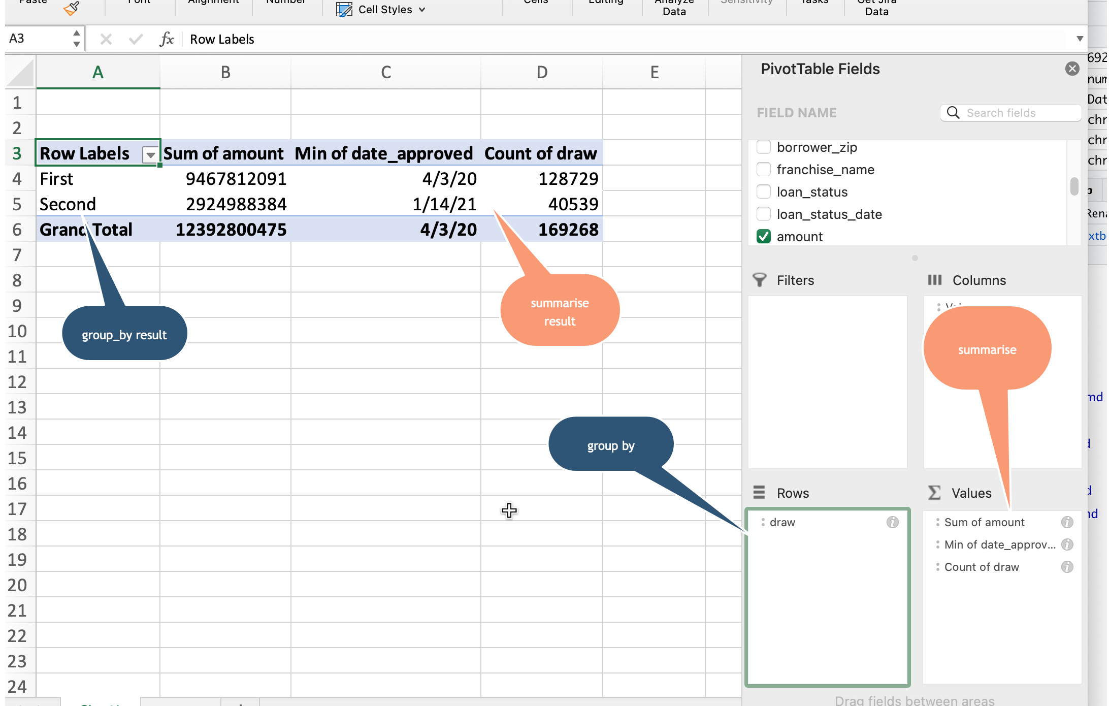
Now that you know how to summarize the whole data frame, you’ll want to start getting totals by category. This is the same thing as a pivot table in spreadsheets: the column names that create the “groups” are the equivalent of the Rows area a spreadsheet pivot table:

Grouping by one column

In the PPP data, the “draw” refers to which of the two programs was involved - the original one created in April 2020, or the one with stricter criteria passed by Congress that December.

Here’s how we’d get some key statistics by draw:

ppp_orig |>
  group_by ( draw ) |>
  summarize ( first_loan = min ( date_approved ), 
              total_amount = sum (amount), 
              total_forgiven = sum (forgiveness_amount, na.rm=T), 
              `# of loans` = n() 
  )

Here are a couple of things to note about grouped output:

• The only columns saved are the ones that are shown in either the group_by or summarize rows. All of the other original columns have been eliminated. You no longer have them to work with .
• The names of the columns for the summary statistics are the ones defined before the “=” sign in the summarize statement.
• TRAP! Don’t ever name your summary columns the same thing as a group_by column. It will override those names, and your output will be unintelligible.

Naming your columns

Note that the name of the columns doesn’t always follow our standard. In this case, # of loans has a special character and spaces. In order to create or use it, you must enclose them in back-tics (`) or you’ll get an error.

Grouping by more than one column

If you wanted to know the numbers outstanding and forgiven by draw, you could add another column to the group by:

ppp_orig |>
  group_by ( loan_status, draw ) |>
  summarize ( first_loan = min ( date_approved ), 
              total_amount = sum (amount), 
              total_forgiven = sum (forgiveness_amount, na.rm=T), 
              loan_ct = n() 
  )

A shortcut : count()

If all you want to do is count or add by group, you can use the count() function as a shortcut. It does the exact same thing as a combination of group_by() and summarize( n() ) and arrange()` to get the number of items in each category, sorted by the most frequent to least:

ppp_orig |> 
  count ( loan_status, draw, 
          sort=TRUE,
          name = "loan_ct")

New ways to summarize

A new version of the tidyverse, in 2023, has changed some of the options for the summarize() verb that make grouping unnecessary much of the time, but it’s confusing. I’m skipping it for now.

18.3 Using and converting groups

Converting from long to wide data

You’ve looked at different ways to think about data, but when we talk about “granular” data, “database” thinking or “tidy” data, we generally mean we’re working with what some people call “long” rather than “wide” data. That is, there are many rows but few columns.

But your instinct is to want to look at a rectangle of wide data, with the values of one column down the side and another across the top. Helpfully, a function called pivot_wider() does just that – pivots your data from long to wide.¹

Start with a simple query with two grouping columns (note that I’ve called the number of loans loan_ct, so it’s easier to work with later on.

This is really hard to read. Turn it on its head with pivot_wider():

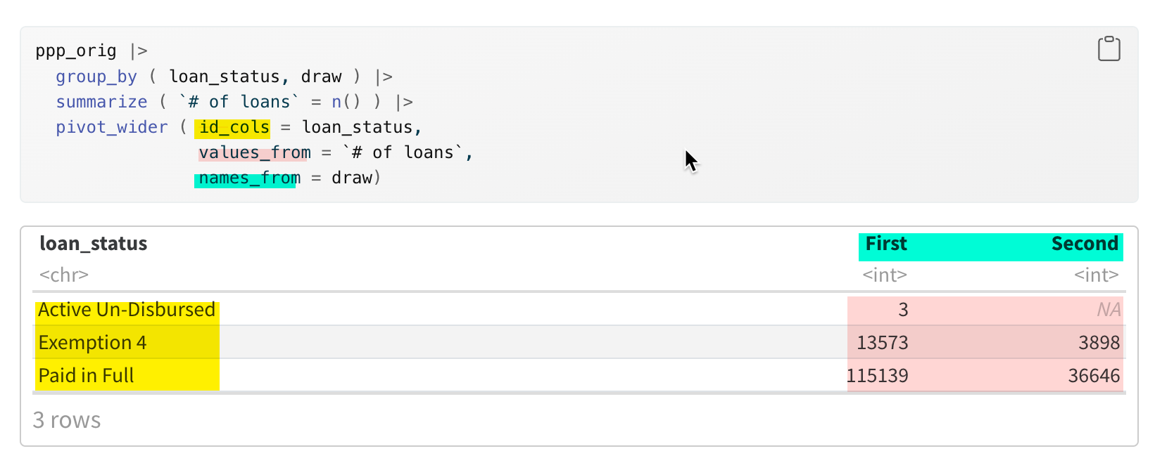
Normally, you’ll only want to have one summary statistic shown in a rectangle, with one column spread across the top and another column shown in rows. There are a lot of advanced options in pivot functions that let you show more than one statistic at a time, and tell R how to name them. There will be a chapter later on that addresses a lot of the problems you have in reading tables, so we’ll put that off for now.

Here’s an explanation of what the command looks like.

```{r}

pivot_wider ( id_cols =  column that you want to see as is down the side,
              names_from =  column with the words you want to see across the top, 
              values_from = column with the numbers you want in the middle
              ) 
```

Tip

Your instinct will be to turn your data into one of these wider tables right from the start, but try to overcome it. The tidyverse expects to do most of its work in “long” format, saving the “wide” format just for printing.

Totals and subtotals

You noticed that when you created the summaries, there was no option to create a “percent of total” such as the percent of loans in each draw, or the percent of money that had been forgiven.

You can use summary functions outside a summarize statement!

This means that you can compute the percent of total, the same way you used an option in pivot tables. This took me a long time to understand, so try to slow down, and just try it a few times! When you look carefully at your output, you’ll start to understand it better.

The trick is to summarize, then use mutate to add a column with the percentages made out of totals:

ppp_orig |>
  group_by ( draw) |>
  summarize ( loan_count = n() ) |>
  mutate ( all_loans = sum (loan_count), 
           pct_of_total = loan_count / all_loans * 100
           )

What happens if you have more than one group?

This is where the idea of grouped data gets a little confusing. It depends on exactly how you did your summarize statement. But if you use the default mechanism, the “all_loans” is the subtotal. The default behavior is that the “groups” are kept for all but the last column listed in the group_by statement, meaning any summaries you do off of the data will refer to the subtotal.

ppp_orig |>
  group_by ( draw, loan_status) |>
  summarize ( loan_count = n() ) |>
  mutate ( loans_in_draw = sum (loan_count),
           pct_of_draw = loan_count / loans_in_draw * 100)

Here’s a pretty typical way to do this: Create a subtotal, use it for your percentages, then pivot the percentages:

ppp_orig |> 
  group_by ( draw, loan_status) |> 
  summarize ( loan_count = n() ) |> 
  mutate ( loans_in_draw = sum(loan_count), 
           pct_of_draw = loan_count / loans_in_draw * 100 ) |> 
  pivot_wider ( 
    id_cols = c(draw, loans_in_draw), 
    names_from = loan_status, 
    values_from = pct_of_draw,
    values_fill = 0)

`summarise()` has grouped output by 'draw'. You can override using the
`.groups` argument.

Now you can easily compare the outcome by draw, by reading across to reach 100% and reading down to compare them.

We’ll have a whole chapter / week on making good tables that are readable and understandable. For now, just remember that it’s always possible to turn a data frame on its head, and that you can compute much of what you need BEFORE you do that.

18.4 Practice

Putting together the grouping and summarizing, along with the commands you learned last chapter to filter, arrange and display the head() and tail() of a dataset should equip you to write the code for these questions:

1. Which lenders provided the most loans?
2. Which lenders provided the most amount of money loaned?
3. Which borrowers got the least amount of money?
4. Show the number of loans in each draw that went to the 24 (including NA) types of businesses. To see them all on one screen, add “, rows.print=25” to the heading of the code chunk like this: {r , rows.print=25}
5. Try to compute the percent of loans that went to projects in each county in Arizona. This will require first filtering, then grouping.

18.5 Postscript: Understanding grouped data

You may have noticed an odd warning after you run the code with multiple grouping columns, for example:

`summarise()` has grouped output by 'draw'. You can override using the `.groups` argument." 

What does that mean?

When you grouped by loan status and draw, R effectively split up your data frame into five independent and completely divorced piles - one for each combination of draw and loan status that it found. It processed them one by one to create the output data frame that was printed out.

After it’s done summarizing your data, R doesn’t know what you want to do with the piles – keep them, or put everything back together again.

By default, after you group by more than one column, it maintains the separate piles for all but the last group in your list under group_by – in this case the loan_status. Here, everything you do after this will work on three piles separately.The message tells you what it did with the piles, and how to change that behavior.

The documentation of grouped data provides details of how each of the tidyverse’s verbs handle grouped data.

Here’s what a “glimpse()” looks like for a data frame that has retained some groups:

ppp_orig |> 
  select ( loan_status, date_approved:amount) |> 
  group_by ( loan_status) |> glimpse()

Rows: 169,259
Columns: 11
Groups: loan_status [3]
$ loan_status      <chr> "Paid in Full", "Paid in Full", "Paid in Full", "Paid…
$ date_approved    <date> 2020-04-10, 2020-04-11, 2020-04-11, 2020-04-29, 2020…
$ draw             <chr> "First", "First", "First", "First", "First", "First",…
$ borrower_name    <chr> "SFE HOLDINGS LLC", "NAVAJO TRIBAL UTILITY AUTHORITY"…
$ borrower_address <chr> "9366 East Raintree Drive", "Po Box 170", "2999 N44th…
$ borrower_city    <chr> "Scottsdale", "Fort Defiance", "Phoenix", "Tucson", "…
$ borrower_state   <chr> "AZ", "AZ", "AZ", "AZ", "AZ", "AZ", "AZ", "AZ", "AZ",…
$ borrower_zip     <chr> "85260", "86504", "85018", "85711", "85250", "85012",…
$ franchise_name   <chr> NA, NA, NA, NA, NA, NA, NA, NA, NA, NA, NA, NA, NA, N…
$ loan_status_date <date> 2021-08-17, 2022-02-05, 2021-09-25, 2021-08-21, 2021…
$ amount           <dbl> 10000000, 10000000, 10000000, 10000000, 10000000, 100…

Notice the “Groups” row at the top – that tells you it’s got three piles, defined by the loan_status column.

Getting rid of the message

You can do two things to get rid of the message. I suggest the first of these, since it makes you explicitly decide what to do each time, depending on your goal:

1. Add a .groups=... argument that looks like this at the end of the summarize statement. This example tells R to do what it does by default, with no warning:

ppp_orig |>
  group_by ( loan_status, draw ) |>
  summarize ( `# of loans` = n() , 
              .groups = "drop_last"
  )

The other possibilities are : .groups="drop" and ".groups="keep" (Note the period before the word “groups”. I have no idea why, but sometimes options are indicated this way.)

2. Add a line to your setup chunk, changing the default behavior through the systemwide options:

   options(dplyr.summarise.inform = FALSE)

What does “tidy” data have to do with groupings?

Grouped data effectively breaks out values of categories and treats them independently, which is the equivalent of temporarily treating them as their own data frame.

It’s somewhat difficult in the tidyverse to summarize across columns – it really wants to summarize rows. In a spreadsheet, it’s just as easy to write an =sum(B1:J1) as it is =sum(B1:B12). That’s not true in R journey so far. This is probably the first time your instinct would be to wreck a perfectly good dataset.

We’ll come back to all of that, but just remember that it’s possible to do all kinds of computations within a group that you’d normally think you want to do across columns. One example is, say, percent change over time. Instead of trying to compute them one by one, you can use groups and the lag() function to do math that depends on a previous row.

state	county	month	cases
AL	Auburn	2020-04-01	24
AL	Auburn	2020-05-01	35
AL	Auburn	2020-06-01	200

covid_data |>
  group_by (state, county) |> 
  arrange (month) |> 
  mutate ( change = cases - lag(cases) , 
           pct_change = change / lag(cases) * 100 ) 

This method will start over for each county, so it will be NA for the first month within each county.

This is just one example of how grouped data is quite powerful when used correctly. There are many others, such as extracting the most recent event in a court history by case. Try to think about how one group would be computed, and then don’t worry how the rest will work – R will do that thinking for you.

---

1. Yes, there is something called pivot_longer(), which lets you turn rectangular data into the tidy form.