2 R Markdown

2.1 Key takeaways

• Markdown makes documenting your work easy
• Formatting commands in Markdown: headings, links, lists and images.
• Adding and running code chunks
• Knitting your markdown into a finished document with code and results.

2.2 Getting started with R Markdown

Creating documents with R Markdown lets you ditch those tiresome data diaries and combine your documentation, code and results all in one, reproducible page. It’s a variant of the markdown language that was was invented as an easy way for early contributors to Wikipedia to author documents that would translate to the web.

In an R Markdown document, write your document around chunks of R code, which integrates your analysis with your writing. (R Markdown is also designed to output your work in other formats, like an actual printed book or slides.) Some news organizations do much of their internal work using R Markdown documents and code.

You must install the rmarkdown package before you can use this feature. Install it in the Console. You only have to do this once on each computer, or in each project on rstudio.cloud:

  install.packages("rmarkdown")

Unlike other packages, it’s automatically loaded when you start up R Studio.

2.3 The anatomy of a document

To format a document, markdown uses simple punctuation to create outline levels, lists, links and other elements of a page.

There are four parts to an R Markdown document:

1. The “front matter”, or YAML.
2. Document features, like text, images, or other elements that you would normally put in an HTML page, but formatted using the easier markdown method.
3. Code chunks – your R computer code.
4. The results of code chunks - what you get back when you execute the code.

2.3.1 Writing in markdown

The document part follows a few basic rules. This markdown cheatsheet from Adam Pritchard goes through them, but the most common are:

Symbol	Format	Comments
#	First level outline	Be sure to follow these marks with a space
##	Second level outline	… and so on
*	A bulleted list item	Separate from the text by one empty line
1	A numbered list
[]()	A link	[my link words](http....)
![]()	An image link	
<>	A simple link shown as an address	<https/cronkitedata.github...>
**	Bold text	**This would be bold**
*	Italic text	*This would be italic*

Front matter / YAML at the top

The way the R knows how to process the page is by reading the very top of the file and looking at the section between three dashes. This is called YAML, or front matter, and it’s extremely picky.

The good news is that the YAML is created for you when you create a new R Markdown document. When you get more comfortable, you may want to tweak the look and feel of your document by adding parts to this section.

---
title: "Title for your page"
author: "Sarah Cohen"
date: "1/6/2020"
output: html_document
---

2.4 Knitting your document

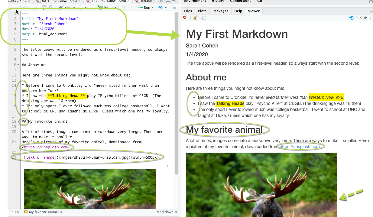
Look at the top of your screen, and you’ll see a knitting needle and the word, “Knit”. Pressing that button will convert your markdown into the finished document.

Here’s how it looks pre-knitted and after knitting:

There are three reasons it might not work:

1. You haven’t saved the document yet.
2. There is an error in that top YAML section. Just copy one that works and try again.
3. There is an error in your R code. (You’ll see how to skip a chunk with an error later on.)

I usually change one default option: I have a large screen so I like to see my document in RStudio rather than as a separate document so I don’t have to flip back and forth between windows. To do that, change the options by clicking on the little gear near the knit button:

2.5 Including R code and its results

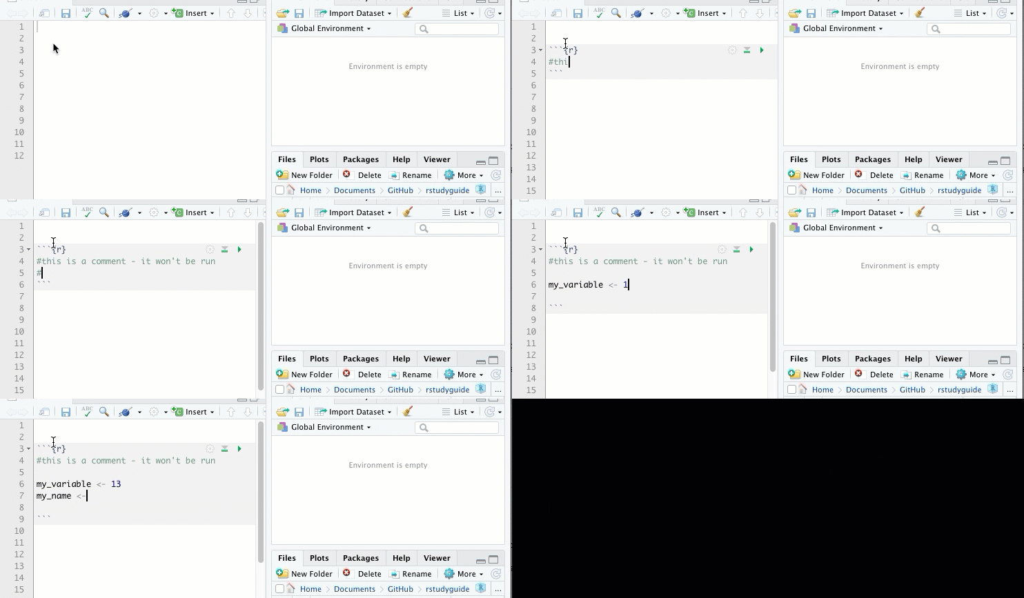
So far, this is just a simple document. It doesn’t contain any R code. To add code, you insert a “code chunk”. You can add it by clicking the +Insert button at the top of the document, or by pressing Option/Alt-Cmd-i Add your code in the gray area between the triple-backtic symbols. Run the code chunk by pressing the arrow button within it, or by pressing Cmd/Ctl-Shft-Enter (either Cmd or Ctl)

Here’s how it works. Notice that when I just typed my_name, the value of that variable is printed just below the chunk:

#this is a comment - it won't be run

my_variable <- 13
my_name <- "Sarah"

my_name

## [1] "Sarah"

This might not seem like much, but think about how it helps you do your analysis. You can write all of your notes right where you do the work. You don’t have to copy and paste information from one place to another, or share out-of-date spreadsheets with your teammates.

2.6 R Markdown starts from scratch

Every time you close down your computer or restart R, you have to run every code chunk to get back to where you left off. This includes loading any libraries and data. This is actually good – it ensures that your project is reproducible.

For long programs or working on complicated datasets, you might split your analysis into several of these programs, saving interim versions of the data as you go along.

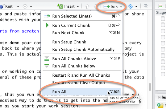
Make sure, though, that you run every part of your document every time you re-open it. The easiest way to do that is to get into the habit of running all chunks as soon as you start your work session using the menu or using Alt-Cmd-R, or through the Run menu:

runall

2.7 RMarkdown resources and exercises

Resources

• “Data driven docs” walkthrough on DS4PS (or, Data Science for the Public Sector)
• RStudio has a quick tour of R Markdown that goes through more than you even need. It goes a little fast.

Exercises

Make sure you have already installed the rmarkdown package before going further.

Create a new R Markdown document with the following elements:

• Front matter with your name, the date and a title for your page.
• A heading introducing a subtopic
• Within that heading, a list of three things about yourself or about a topic you love, in a bulleted list.
• Another heading
• An image that you like (you’ll have to save it in your project.)
• Another heading
• A code chunk, in which you create a variable and assign it a value.

Then knit the document and compare the sections.

2.8 Bonus: Styling your R Markdown documents

Once you’re familiar with R Markdown and comfortable with it, you’ll probably want to make your documents look a little more 21st century than the default. Here are a few things you can do to make it look better:

You can change most style options of a document through the YAML front matter that we’ve largely left alone so far. When you create a new document, that front matter is created for you between three dashes at the top. It might usually look like this:

  ---
  title: "My title"
  author: "My name"
  date: "1/24/2020"
  output: html_document
  ---

This section is really picky, which is why we’ve left it alone so far. But you can change several styling options very easily if you’re careful.

Among the most simple things to change are:

• A new theme with more modern colors and fonts.
• Tables that are “paged” rather than simple text output
• A table of contents for links to each heading.

Without doing much else, you can change the look and feel of the knitted document by using free Bootswatch themes (toward the bottom of the page on the bootswatch site). You’ll have to be careful changing the front matter when you use them – it’s very sensitive to exact syntax, including indentation.

This example does three things:

1. Uses the “journal” theme from Bootswatch

2. Creates a table of contents that goes to the 2nd outline level (## in your markdown)

3. Prints tables in a more fancy way, that pages both vertically and horizonatally. Just be careful with this: It will print up to 10,000 rows, even if you can’t see them, bringing your browser to a halt pretty quickly.

      ---
      title: "My title"
      author: "My name"
      date: "1/24/2020"
      output: 
         html_document:
            df_print: paged
            theme: journal
            toc: true
            toc_depth: 2
      ---

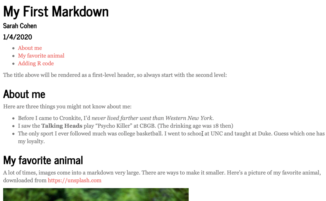
Here’s a preview of what my example markdown would look like with these options:

journal example with toc

There are a lot of other ways to style these documents using other packages. A few you might look into if you’re interested:

• prettydocs, which tries to match up with the default Github Pages themes.
• kable and kableExtra to work with styling tables.
• DT datatables that latches into the Javascript DataTables library, making sortable, searchable tables with tight control over formatting. (Not for the faint of heart if you don’t already know Javascript.)